In the second quarter of my Master’s program, I had a professor who really emphasized the importance of writing modular code and testing each function that you write. The way he graded our weekly assignments was by running each function with every type of input your function should be able to handle. So, it was in our best interests to make sure that every branch of our functions worked correctly. As a result, I wrote a lot of tests.
After his class ended, I often thought about writing test statements, but doing so was never required again in any of my other classes, and from the lack of online literature surrounding testing for data science, I had just assumed that it wasn’t something data scientists do. Sure, I would casually test the output of functions at the console after writing them to ensure they worked as expected, and I would throw in stopifnot statements on occasion, but I had never been disciplined about it. Until now.
Since the compatibility quiz was fresh on my mind, I decided to supplement tests for this short script using the testthat package. I used this guide to get started, and I used the tests he wrote for dplyr as another reference.
The recommended style is to not have all of your tests in one test file, but since my script was pretty short, I felt it was fine to do. The workflow that I am going to start trying out is to write tests in separate tabs as I am working on the actual code for the analysis/model. The test file is just composed of a series of related test_that statements. For example, here is one of my test statements:
test_that("to_sentiment_score returns the correct word count",{expect_is(to_sentiment_score("something"),"integer")expect_equal(to_sentiment_score("something or another"),3)expect_equal(to_sentiment_score(NA),-1)})
I saved this in a folder called tests (make sure to start the name your file with test) and I run all of my test statements using test_dir("tests/"). That’s all! Super simple to get going.
While I was creating the test suite, I noticed that I had already written a few error messages within my functions. I think it’s worthwhile to have both - one as an intermediate check and one to as a final check on the output. Also, for a few of the statements, I felt they were kind of redundant as I was writing them, especially since I had already seen the result. However, then I realized that testing is not just to guarantee the accuracy of your code at the time, but it’s also to ensure your future changes don’t affect the integrity of your results.
All in all, I’m surprised that testing is not more recommended in data science, especially since errors are just as, if not more likely, to creep up when dealing with numbers in this field than in engineering, where testing is an integral part of development. I wish I could go back in time and tell my past self to do this, but since that’s impossible, I hope this post has encouraged you to get started with testing!
If you have any feedback or questions for me, please shoot me an email at melodyyin18@gmail.com. Thank you!
Remember those quizzes that we used to take in middle school and/or high school? I remember filling out a set of questions in homeroom and receiving a short list of people that I was most compatible with and another list with my least compatible matches. These quizzes were always entertaining and my friends and I would have a lot of fun completing them and comparing our results. So, I thought it would be a great way to build camaraderie in the office and help people to get to know each other. Plus, for an extra layer of fun, I could design my own algorithm!
I went to our Office Manager, Kelly, with the idea and she was on board and just as excited as I was! We sat down with a couple of our other coworkers and created 25 questions using Google Forms. Some were multiple choice, others were on a linear numeric scale, a few were checkboxes and the last question was a short answer. The idea was to use a person’s response to determine everyone else’s relative distances, and select the top 3 closest individuals as that person’s matches. We also later decided to include the furthest match, because opposites attract, right?
To determine distance, I needed to convert all responses into some type of numerical representation, because there’s no way to find how far apart someone who chose choice A is from someone who chose choice C when the choices are categorical. On the other hand, if the choices could be converted into numerics then the multiple choice or checkbox question essentially becomes a linear numeric scale question and deriving the distance is quite straightforward. So, I sat down with Kelly again to choose a few of appropriate questions and converted their text choices to numbers. For example, one of our questions was: “Which distribution center would you work in if you had the choice?”, and we ranked the answers by distance from San Francisco.
For the remaining questions, I assigned a binary vector to each possible response. For example, if someone chose choice B and C in a checkbox question with 5 potential choices, their binary vector would be: [0 1 1 0 0]. Similarly, if someone chose choice D in a multiple choice question with 4 choices, their vector would look like: [0 0 0 1].
Next, I had to choose a distance measure that was able to handle 0/1 values appropriately, and decided on the binary/Jaccard distance, which is included in base R’s dist function. For multiple choice questions, using this distance measure meant that those who chose the same answer would have the distance 0, and those who did not would have distance 1. It worked similarly for checkbox questions, except the resulting distance could range between 0 and 1 depending on the length of the vector and the number of overlapping positions.
I had originally planned on doing sentiment analysis on the response to the short answer question, but didn’t feel it was worthwhile to spend time stemming the words, especially since most people skipped the question! Instead, I opted for a simple word count to quantify the responses to this question.
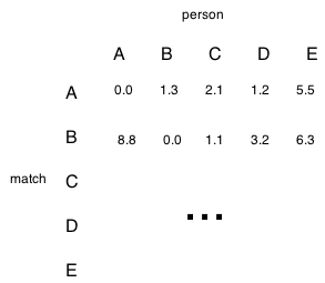
Now, each question has an n-element vector of everyone’s responses, where n is the number of participants in the quiz. Since the questions are on different scales, we normalize the responses for each question to give every one the same weight. Then, all of the matrices are summed and the final matrix looks like this:
So, we can see that the best match for person A is D and the best match for person B is C.
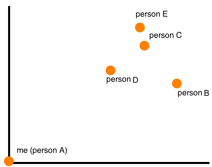
A plot of the distances can also be generated. Since distances are all relative (e.g., your distance from me is relative to where I am), each person has their own plot where they are at the origin, and it looks something like this:
Out of the 70-something people in the office, 60 people filled out the quiz and received their top 3 matches as well as their worst match. Although everyone had matches, there were around 10 people who did not show up in anyone else’s top 3. Conversely, there were a few people who dominated the worst match list, with yours truly ranking at #3 in frequency of appearance in worst match list (the irony!!! betrayed by my own algorithm :c). Overall, it was a success!
The code for the entire quiz plus the compatibility plot can be found here.
Lastly, this blog just turned 1 year old! In the past year, I wrote 11 posts and created 5 statscapades. This year, I aim to double that amount!
If you have any feedback or questions for me, please shoot me an email at melodyyin18@gmail.com. Thank you!
1. Use RStudio I was introduced to R in a regression course in my junior year of college. The professor used RGUI, so that’s what I used as well. I didn’t hear about RStudio until the following year in Statistical Computing - but being the skeptic I am, I thought it was just a bulkier version of RGUI. It stuns me to think that I went through nearly 2 years of being a useR (including an internship where my main tool was R) before I downloaded RStudio. There are so many advantages of RStudio I won’t list them here, but if you haven’t made the switch…. DO IT NOW!!! Their newest release (v0.99.879) also contains significant improvements!
2. Use knitr I can’t be the only one who was either (1) attaching raw R code along with my graphs and written reports, which I usually created in (gasp) Word or (2) copying and pasting screenshots of code in reports when the person reading it is liteRate. Not only were these reports ugly and a hassle to make, but they were difficult for people to read as well as for me to review. Thankfully, I now use knitr to generate reports and presentations (using ioslides), so those problems are no more! Additionally, writing reproducible code has made me a better analyst.
3. Use dplyr What was I doing before dplyr? I load this package at the start of every script I write. I have the laptop sticker. Exploratory analysis is so much more efficient (and readable) using this package vs. the base functions. Every analyst needs to use this.
4. Use ggplot2 properly I also have this laptop sticker. I have to admit, for the longest time I was just throwing ggplot code together and hoping for the best, making visualizing results much more troublesome than it really should have been. Reading the docs is super helpful, and I do think the authors tried to make things as straightforward as possible. A realization that helped me better understand the package is that it works in layers. Every function you + to the ggplot() call is another layer you are placing on your graph.
5. How to select columns by name Not sure if this is something I should’ve learned long ago, but I never knew how to select a column within a dataframe by the (string) name. I’ve always done df$my_column or df[,col_position_of_my_column]. Recently, I learned that you can also do df[[str_name_of_my_column]]. I feel better now.
6. Declare default parameters in functions Pretty self-explanatory. I like that this keeps your code clean and helps debugging. For example:
some_function=function(train=training_set,test=testing_set,res=data.frame()){# do something
return(res)}# I call this normally
x=some_function()# but I can also do this if I want to test on a subset of the training/testing set
x=some_function(training_subset,testing_subset)
7. Debug Breakpoints are really useful when I know the general area where the bug is occurring and want to check out the relevant variables at that point in the code. I’ve also been adding stopifnot statements in scripts, and doing this has been tremendously helpful in helping me catch mistakes that would otherwise go undetected (well, that is, until my manager gets back to me… :)). At some point, I want to check out the testthat package too.
8. xapply functions, do.call xapply becomes really important when working with large datasets, and they’re much more concise than repeating code or writing loops. An useful application is calling sapply(df, is.numeric) when you want to find the numeric columns… very handy for cleaning training data with many predictors. I haven’t had much practice working with mapply or Map, but they’re in the toolbox…
I think of do.call as the opposite of lapply. While do.call sends your list into the specified function, lapply distributes your function to each element in the list.
9. Dealing with NAs The datasets provided in university courses are always cleaned, so you never really have to deal with missing values or do data integrity checks. However, these issues are almost always present in datasets you’d encounter in another setting. I now always use the na parameter (in the readr package) when reading in data. I also use anyNA for doing quick checks and replace_na (in the tidyr package) and na.omit for handling NAs.
10. Git locally THIS IS AWESOME. I didn’t know version control was possible without pushing to a public repo until recently. No more saving R files with the dates at the end… or scrolling through a script trying to remember which line I changed last week… The interface RStudio provides is actually super straightforward - it doesn’t require any knowledge of git commands. All you need to do is check your files, write a commit message, and press a button!
I consider myself proficient in R but there’s still a lot for me to learn. Looking forward, I want to build a Shiny app, create a package, and become more involved in the useR community here in the Bay Area. I’ve definitely had my share of frustrations working with these tools/packages/functionalities, so to all the R beginners out there who were in my position: don’t give up!!!
If you have any feedback or questions for me, please shoot me an email at melodyyin18@gmail.com. Thank you!